- Home
- Table in APA Format
- Correlation Table Examples
- Correlation Analysis
What Is Correlation Analysis?
Correlation analysis is a statistical method used to examine the relationship between two variables.
Despite its technical name, its main purpose is usually quite simple.
Correlation analysis helps you determine whether two variables are related and, if they are, the direction and strength of that relationship.
A Simple Example of Correlation Analysis
Imagine you want to examine whether the number of hours students study each week is related to their final examination scores.
You collect information from 80 students. You record:
- the number of hours each student studies per week
- each student's final examination score
The results are shown in Figure 1. Each point represents one student.
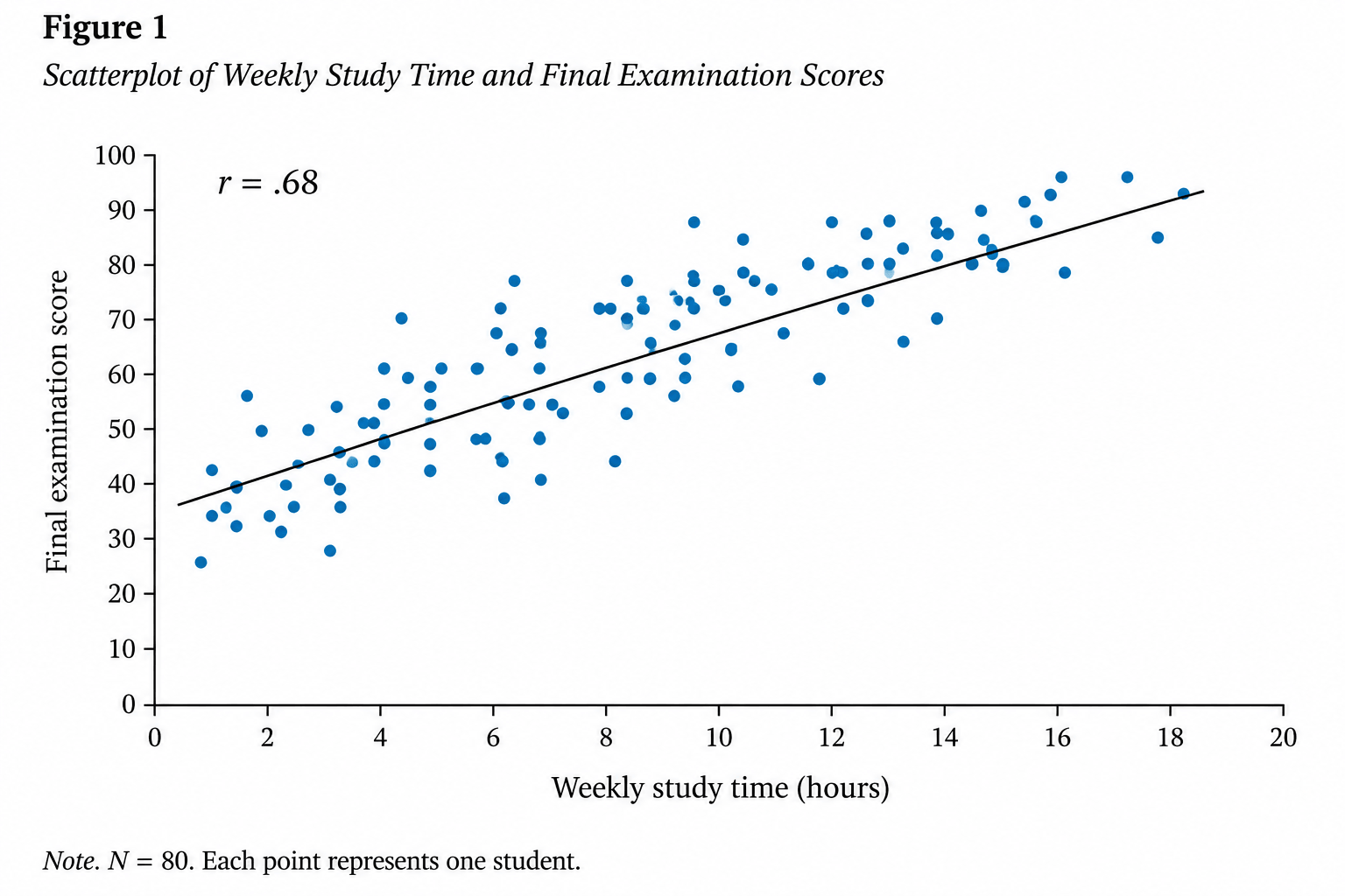 Figure 1: Study Time and Examination Score Correlation
The points generally move upward from left to right.
Students who study for more hours tend to receive higher examination scores.
This suggests a positive relationship between the two variables.
However, the graph alone does not give you a precise measure of the relationship.
Correlation analysis does this by calculating a correlation coefficient.
The Correlation Coefficient
Pearson's correlation coefficient is represented by the statistical symbol r.
The value of r can range from −1 to +1.
In the study-time example, r = .68.
The correlation coefficient tells you two important things:
- the direction of the relationship
- the strength of the relationship
Direction of the Relationship
A correlation can be positive, negative, or close to zero.
Positive Correlation
A positive correlation means that higher values of one variable tend to occur with higher values of the other.
In the study-time example, r = .68.
Students who study for more hours tend to receive higher examination scores.
Both variables tend to move in the same direction.
Negative Correlation
A negative correlation means that higher values of one variable tend to occur with lower values of the other.
For example, suppose you examine the relationship between test anxiety and examination scores and find that r = −.58.
Students with higher test anxiety tend to have lower examination scores.
The minus sign identifies the negative direction of the relationship.
Little or No Correlation
A correlation close to zero indicates little or no linear relationship between the variables.
For example, r = .05 would indicate a very weak linear relationship.
This does not necessarily mean that the variables have no relationship at all. They could have a relationship that is not well represented by a straight-line pattern.
Strength of the Relationship
The size of the correlation coefficient indicates the strength of the relationship.
Ignore the positive or negative sign when considering strength.
For example, r = .70 and r = −.70 have the same strength. One is positive and the other is negative.
As a general guide:
- around .10 indicates a small correlation
- around .30 indicates a moderate correlation
- around .50 or greater indicates a large correlation
These values are guidelines rather than strict rules.
The importance of a correlation depends on the subject being studied and the circumstances in which the results will be used.
In the study-time example, r = .68.
This indicates a relatively strong positive relationship between weekly study time and examination scores.
Perfect Correlations
A correlation of +1 represents a perfect positive relationship.
As one variable increases, the other increases in a completely consistent pattern.
A correlation of −1 represents a perfect negative relationship.
As one variable increases, the other decreases in a completely consistent pattern.
Perfect correlations are uncommon because people and other real-world measurements naturally vary.
Statistical Significance
Correlation analysis also helps you determine whether there is statistical evidence of a relationship beyond the particular sample being studied.
The p value is used for this purpose.
A result is commonly treated as statistically significant when p < .05.
In the study-time example, r = .68, p < .01.
The correlation of .68 tells you that there is a relatively strong positive relationship.
The p value tells you about the statistical evidence for that relationship.
A p value below .01 means that, if there were actually no correlation in the population, a sample correlation this extreme or more extreme would be unlikely to occur through random sampling variation.
This provides strong statistical evidence that study time and examination scores are related.
Statistical significance does not tell you how strong or important the relationship is.
The correlation coefficient and the p value therefore answer different questions:
- r tells you the direction and strength of the relationship.
- p helps you assess the statistical evidence for the relationship.
Why Sample Size Matters
The statistical significance of a correlation depends partly on the number of observations in the analysis.
A relatively small correlation may be statistically significant when the sample is very large.
The same correlation may not be statistically significant with a small sample.
This is another reason why you should not use the p value to judge the strength of a relationship.
Look at the correlation coefficient itself when considering strength.
Examining Several Variables
Correlation analysis becomes particularly useful when you have several variables.
Suppose you extend the study to include:
- weekly study time
- class attendance
- average nightly sleep
- test anxiety
- final examination score
You can calculate a correlation between every pair of variables.
The results are shown in Figure 2. Each point represents one student.
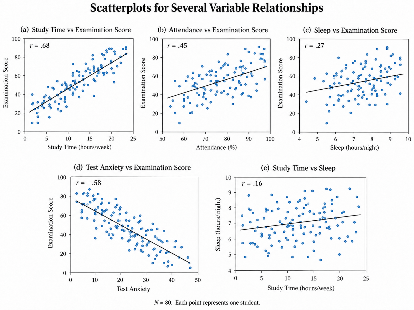 Figure 2: Correlations Among Student Study and Examination Variables
The results show:
- study time and examination score: r = .68
- attendance and examination score: r = .45
- sleep and examination score: r = .27
- test anxiety and examination score: r = −.58
- study time and sleep: r = .16
A correlation table provides a compact way to present all these relationships.
Understanding a Correlation Table
Figure 3 shows the correlation table.
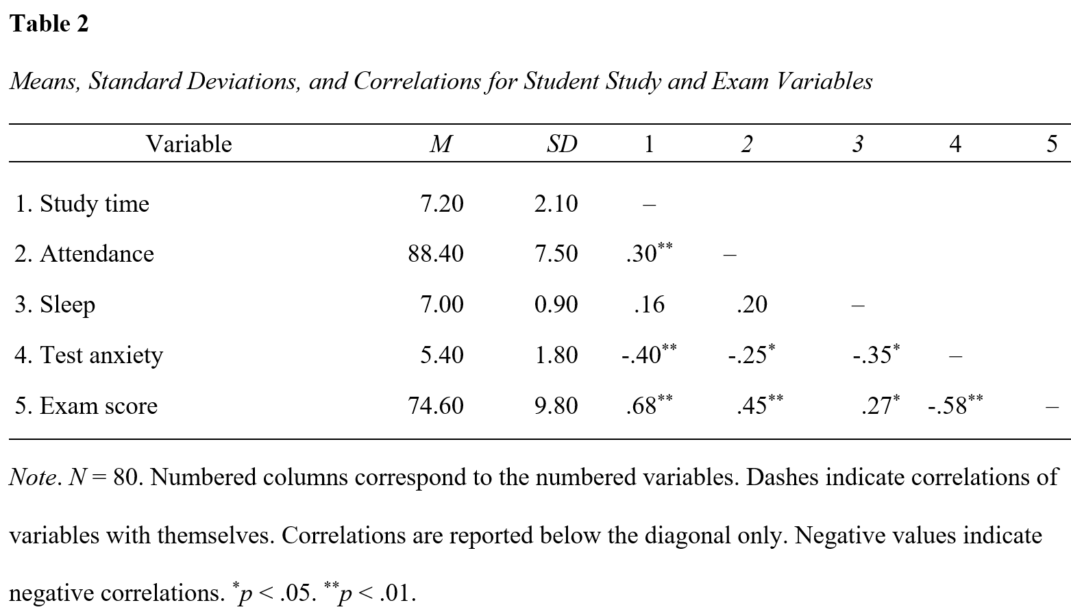 Figure 3: Correlations Among Several Student Variables
The table contains several different types of information.
Variable
Each variable is given a number.
- Study time
- Attendance
- Sleep
- Test anxiety
- Exam score
These numbers are then used as column headings so that the full variable names do not need to be repeated across the table.
M
M represents the mean.
The mean is the average value for the variable.
For example, the mean weekly study time is M = 7.20.
Students therefore studied for an average of 7.20 hours per week.
SD
SD represents the standard deviation.
The standard deviation indicates how spread out the values are around the mean.
For weekly study time, SD = 2.10.
A larger standard deviation indicates greater variation among the observations.
Correlation Coefficients
The numbered part of the table contains the correlation coefficients.
The correlation coefficient is represented by the statistical symbol r.
For example, look at row 5 for exam score.
The value under the column headed 1 is .68**.
That column represents study time.
The correlation between study time and examination score is therefore r = .68.
The positive value indicates a positive relationship, and the size of .68 indicates a relatively strong relationship.
Positive and Negative Values
Positive values indicate positive correlations.
For example, r = .45 for attendance and examination score means that students with higher attendance tend to receive higher examination scores.
Negative values indicate negative correlations.
For example, r = −.58 for test anxiety and examination score means that students with higher test anxiety tend to receive lower examination scores.
Asterisks
Asterisks beside a correlation coefficient indicate statistical significance.
Statistical significance means that a result is unlikely to have occurred just by chance if there were really no relationship in the population.
For the p value, a lower number means stronger evidence against the idea that the result occurred by chance.
For example, p = .01 provides stronger evidence than p = .04.
A common cutoff is p < .05 for statistical significance.
The asterisks and the table note indicate the statistical significance.
For example, .27* in Figure 3 indicates a correlation of .27 that is statistically significant at p < .05.
The value .68** means that the correlation is .68 and is statistically significant at p < .01.
A correlation without an asterisk, such as .16, does not meet either of the significance levels identified in the table note.
The asterisks indicate statistical significance. They do not indicate the strength of the correlation.
The Diagonal
A variable is perfectly correlated with itself.
For example, the correlation between study time and study time would always be r = 1.00.
These values do not provide useful information, so the diagonal cells are commonly shown with an em dash rather than 1.00.
Why Is Only Half of the Table Filled?
The correlation between two variables is the same whichever way you look at it.
For example:
- the correlation between study time and examination score is .68
- the correlation between examination score and study time is also .68
There is no need to report the same value twice.
For this reason, correlation tables commonly show the coefficients either below or above the diagonal and leave the other half blank.
A Scatterplot Helps You See the Relationship
A scatterplot provides a useful visual representation of a correlation.
Each point represents one observation.
For the student example:
- weekly study time appears on one axis
- examination score appears on the other
- each point represents one student
When the points generally rise from left to right, the relationship is positive.
When they generally fall from left to right, the relationship is negative.
When the points show no clear linear pattern, the correlation will usually be closer to zero.
The more closely the points follow a straight-line pattern, the stronger the linear correlation tends to be.
Outliers Can Affect a Correlation
An outlier is an observation that differs substantially from most of the other observations.
For example, imagine that one student studies for many more hours than everyone else but receives an unusually low examination score.
That single observation could affect the correlation coefficient.
You should therefore examine the data, often with a scatterplot, rather than relying only on the value of r.
Correlation Does Not Prove Cause and Effect
A correlation shows that two variables are related.
It does not, by itself, show that one variable causes the other.
In the study-time example, students who study for more hours tend to receive higher examination scores.
However, you cannot conclude from the correlation alone that additional study caused the higher scores.
Other factors may be involved. For example, students who study more might also:
- attend more classes
- be more motivated
- have better previous achievement
- use more effective study methods
Describe correlation results using expressions such as:
- is related to
- is associated with
- has a positive correlation with
- has a negative correlation with
Avoid saying that one variable causes another unless the research design provides evidence for a causal conclusion.
Correlation and Regression
Correlation and regression both examine relationships between variables, but they answer different questions.
Correlation describes the direction and strength of the relationship between two variables.
For example, r = .68 describes the relationship between weekly study time and examination score.
Correlation treats the two variables symmetrically. It does not designate one as the predictor and the other as the outcome.
Regression analysis goes further by using one or more predictor variables to estimate or help explain an outcome.
For example, regression can estimate how much the predicted examination score changes for each additional hour of weekly study.
See Regression Analysis for a fuller explanation.
Calculating Correlations
In practice, statistical software normally calculates correlation coefficients and p values for you.
Programs such as IBM SPSS Statistics and jamovi can calculate correlations among two or more variables and produce the information needed for a correlation table.
You do not need to calculate the correlation coefficient yourself to understand what the results mean.
The important points are:
- the sign of r shows the direction of the relationship
- the size of r shows the strength of the relationship
- the p value provides information about statistical significance
- a correlation does not by itself establish cause and effect
For examples showing how to present these results, see Correlation Table in APA Format.
Summary of Correlation Analysis
Correlation analysis examines relationships between variables.
Pearson's correlation coefficient, r, ranges from −1 to +1.
A positive value indicates that the variables tend to move in the same direction. A negative value indicates that they tend to move in opposite directions.
The size of the coefficient indicates the strength of the relationship. Values closer to −1 or +1 represent stronger linear relationships, while values closer to zero represent weaker linear relationships.
The p value helps you determine whether the correlation is statistically significant.
A correlation table allows you to present correlations among several variables in a compact form, often together with their means and standard deviations.
Correlation analysis can identify relationships between variables, but it does not by itself establish cause and effect.
Frequently Asked Questions
Can I use correlation when the two variables use different units?
Can I use correlation when the two variables use different units?
Yes. The variables do not need to use the same units. For example, you can correlate hours of study with an examination score expressed as a percentage.
Does changing the units of measurement change the correlation?
Does changing the units of measurement change the correlation?
No. Changing from hours to minutes, for example, does not change the correlation coefficient.
When should I use Pearson's correlation?
When should I use Pearson's correlation?
Pearson's correlation is generally used when you want to measure the linear relationship between two numerical variables.
What is Spearman's correlation?
What is Spearman's correlation?
Spearman's correlation is an alternative to Pearson's correlation. It is commonly used with ranked or ordinal data, or when the assumptions for Pearson's correlation are not appropriate.
Can two variables have a relationship even when the correlation is close to zero?
Can two variables have a relationship even when the correlation is close to zero?
Yes. Pearson's correlation measures a linear relationship. Two variables can have a strong curved relationship and still have a correlation close to zero.
Can a correlation be calculated if some data are missing?
Can a correlation be calculated if some data are missing?
Yes, but the way missing values are handled depends on the statistical software and the method selected. The number of observations used for different correlations may therefore vary.
Can I compare two correlation coefficients just by looking at their values?
Can I compare two correlation coefficients just by looking at their values?
You can compare their apparent strength, but you should not assume that two correlations are statistically different simply because their values differ. A statistical test is needed to determine whether the difference is significant.